
|
The October data from the latest CSA surveying experiment arrived via email at CSA's offices in January. The coordinates for each survey point were included, and there was a file with the coordinates for each day's work. In fact, there were multiple files for each day's work, each in a different format. We already had our field notes, but the coordinate information had required processing by the surveyors in Athens before it could be used.
In many cases the coordinates for a given point provided only a part of the needed information because we often surveyed the corner of a block by surveying multiple points, none of which lay at the actual corner. This was necessary when the corner itself had been abraded or otherwise damaged so that a direct measurement was impossible. The photograph in Figure 1 illustrates such a block. The corner itself is no longer present; instead, there is now a gap. The original corner (at D) can be determined, though, by surveying three separate points, one for the width (the x-coordinate -- A), one for the depth (the y-coordinate -- B), and one for the height (the z-coordinate -- C). This process mirrors the way one would determine 3D coordinates with a conventional approach using tape measures, line levels, and the like -- a separate measurement for each coordinate. So long as the x-coordinate is taken for a point vertical to the actual corner, the x-value should hold. So long as the z-coordinate is taken for a point horizontal to the actual corner, the z-value should hold. Similarly, so long as the y-coordinate is taken for a point at the same depth as the corner, the y-value should hold.
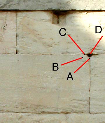 | Figure 1. Coordinates from points A, B, and C, were substituted for those of missing corner D. |
The coordinates for the Propylaea work in October were expressed in the original coordinate system established by the surveyor and related to the Acropolis generally. However, the point coordinates had to be available to the project in a coordinate system with the x-axis parallel to the wall on which the survey points were taken. Otherwise, the y-value would not remain constant if the surveyed point was not at the corner. (If the reason for this is not clear to you, please select explanation to step out of this narrative for an explanation. This may tax your memory of high-school geometry.)
Given the problem with coordinate systems, our first task was to translate the survey information from the original coordinate system used by the surveyor to the wall-based coordinate system with the x-axis parallel to the wall (actually two wall-based coordinate systems, one with the x-axis parallel to the east wall and one with that axis parallel to the south wall). This was a multi-step process. First, the original coordinates -- in text files, as received from Manolis Kapokakis, the surveyor who has worked so well with us in Athens -- were compiled into a single file (with a text editor) and then put into a spreadsheet where a series of AutoCAD commands could be created by formula. The commands were designed simply to place text (the survey point number) at the point in the model indicated by the original coordinates. Then the series of AutoCAD commands was copied and pasted into the AutoCAD command line to create in our AutoCAD model each of the text entries at the appropriate spot.
The starting text file looked like this:
| 1<tab> | 107.998<tab> | 107.428<tab> | 101.966<cr> |
| 2<tab> | 108.263<tab> | 107.409<tab> | 102.336<cr> |
| 3<tab> | 108.628<tab> | 107.431<tab> | 101.973<cr> |
| 4<tab> | 107.376<tab> | 107.425<tab> | 101.961<cr> |
| 5<tab> | 108.001<tab> | 107.433<tab> | 101.534<cr> |
| 6<tab> | 107.376<tab> | 107.425<tab> | 101.962<cr> |
| 7<tab> | 106.749<tab> | 107.432<tab> | 101.464<cr> |
| 8<tab> | 107.375<tab> | 107.430<tab> | 101.468<cr> |
| . . . |
(The <tab> and <cr> indicators for tab and return characters are included because the actual characters, not these indications of their presence, are critical to moving the data into a spreadsheet.) Saved as a simple text file (.txt), the file could be opened with a spreadsheet. The initial spreadsheet looked very much the same, just a list of point numbers and coordinates, but they were in columns:
| Point number | X-coord. | Y-coord. | Z-coord. |
| 1 | 107.998 | 107.428 | 101.966 |
| 2 | 108.263 | 107.409 | 102.336 |
| 3 | 108.628 | 107.431 | 101.973 |
| 4 | 107.376 | 107.425 | 101.961 |
| 5 | 108.001 | 107.433 | 101.534 |
| 6 | 107.376 | 107.425 | 101.962 |
| 7 | 106.749 | 107.432 | 101.464 |
| 8 | 107.375 | 107.43 | 101.468 |
After the data had been put into the spreadsheet, an equation was constructed to fill the fifth column with the actual AutoCAD commands. That equation put into the fifth column the following: the word "text" plus a space (needed to activate the command in AutoCAD) plus the three coordinates (separated by commas) plus 3 spaces (to push AutoCAD through the sequence of questions about text size and angle) and the number of the point (from column one), which would become the text in the model. (The formula -- for Excel -- was this for row N, column E: ="text "&BN&","&CN&","&DN&"[3 spaces]"&AN - "text and a space plus the value in col. B, row N as text, a comma, the value in col. C, row N as text, another comma, the value in col. D, row N as text, 3 spaces, and the value in col. A, row N as text.) The spreadsheet then looked like the following (with <space> and <3 spaces> used instead of the actual spaces):
| Point Number |
x-coord. | Y-coord. | Z-coord. | AutoCAD command |
| 1 | 107.998 | 107.428 | 101.966 | text<space>107.998,107.428,101.966<3 spaces>1 |
| 2 | 108.263 | 107.409 | 102.336 | text<space>108.263,107.409,102.336<3 spaces>2 |
| 3 | 108.628 | 107.431 | 101.973 | text<space>108.628,107.431,101.973<3 spaces>3 |
| 4 | 107.376 | 107.425 | 101.961 | text<space>107.376,107.425,101.961<3 spaces>4 |
| 5 | 108.001 | 107.433 | 101.534 | text<space>108.001,107.433,101.534<3 spaces>5 |
| 6 | 107.376 | 107.425 | 101.962 | text<space>107.376,107.425,101.962<3 spaces>6 |
| 7 | 106.749 | 107.432 | 101.464 | text<space>106.749,107.432,101.464<3 spaces>7 |
| 8 | 107.375 | 107.43 | 101.468 | text<space>107.375,107.43,101.468<3 spaces>8 |
Each cell of the rightmost column thus contained an AutoCAD command to enter the text -- the ID numbers - - at the point indicated by the original coordinates -- exactly as it might be entered into the command line of AutoCAD. The entire column of the spreadsheet could then be copied and pasted into the AutoCAD command line. In an instant all the points surveyed -- more than 1600 of them -- were in the model. The process did not require that any coordinates ever be typed; all were taken from one file format to another.
At the conclusion of that operation all the points from the survey had been placed into the model, but all were entered with the original coordinate system in use by the surveyor, not the wall-based coordinate systems required for this work. The next step was to translate the survey coordinates into the wall-based coordinate systems -- two such wall-based coordinate systems, one with the x-axis parallel to the south wall and one with the x-axis parallel to the east wall. Fortunately this is relatively easy with AutoCAD. It could be done quickly and easily -- and temporarily so that the original coordinate information was never changed. (AutoCAD can set up any number of temporary user coordinate systems -- grids with different 0,0,0 points and different orientations -- with a fairly simple command sequence. This is one of AutoCAD's most valuable features but also one very difficult to learn. Knowing this would be necessary, we had specifically surveyed two points to be used to define the x-axis for the east wall and two others for the axis of the south wall.) When one of the new wall-based coordinate systems was in use, any query of the data produced coordinate information in terms of that coordinate system. Thus, a listing of the points previously entered could be created with all the point coordinates expressed in one of the wall-based coordinate systems. AutoCAD not only made it possible for us to list the points, but a simple command made the program save all text output during the current AutoCAD session in a log file. The file included all the coordinate information for each point - expressed in the wall-based coordinate system - and extraneous text, but it was easy to load the portion of the log file with the coordinate information into a text editor and remove all the extraneous text. A series of find-and-replace commands did that quickly. The listing for three points was as follows (formatting will not show properly because of HTML conventions), showing the three coordinates and the actual text (all in boldface here), which is the ID number for the point located at those coordinates:
| TEXT | Layer: "south wall - orig" |
| Space: Model space | |
| Handle = 1B0E | |
| Style = "Standard" | |
| Font file = txt | |
| start point, X= -0.2192 Y= -0.0591 Z= 5.3930 | |
| height 1.0000 | |
| text 327 | |
| rotation angle 180 | |
| width scale factor 1.0000 | |
| obliquing angle 0 | |
| generation normal |
| TEXT | Layer: "south wall - orig" |
| Space: Model space | |
| Handle = 1B0D | |
| Style = "Standard" | |
| Font file = txt | |
| start point, X= -0.2332 Y= -0.0551 Z= 5.3900 | |
| height 1.0000 | |
| text 326 | |
| rotation angle 180 | |
| width scale factor 1.0000 | |
| obliquing angle 0 | |
| generation normal |
| TEXT | Layer: "south wall - orig" |
| Space: Model space | |
| Handle = 1B10 | |
| Style = "Standard" | |
| Font file = txt | |
| start point, X= -0.1672 Y= -0.0583 Z= 5.0800 | |
| height 1.0000 | |
| text 329 | |
| rotation angle 180 | |
| width scale factor 1.0000 | |
| obliquing angle 0 | |
| generation normal |
Two search-and-replace commands (plus removing the first and last portions of the excess) yielded this text:
X= -0.2192 Y= -0.0591 Z= 5.3930
height 1.0000
text 327
X= -0.2332 Y= -0.0551 Z= 5.3900
height 1.0000
text 326
X= -0.1672 Y= -0.0583 Z= 5.0800
height 1.0000
text 329
Another search-and-replace command removed the unwanted height specification (referring to the height of the text in the CAD file) as well as the "text" notation, replacing them with a tab character (<cr> for carriage return is shown here for the first time, but the actual characters had been present previously):
X= -0.2192 Y= -0.0591 Z= 5.3930<cr>
<tab> 327
X= -0.2332 Y= -0.0551 Z= 5.3900<cr>
<tab>326
X= -0.1672 Y= -0.0583 Z= 5.0800<cr>
<tab>329
Four more find-and-replace commands removed the "X=," "Y=," and "Z=" text plus associated spaces, and a final command replaced the <cr> <tab> sequence with only <tab>:
-0.2192<tab> -0.0591<tab> 5.3930<tab> 327
-0.2332<tab> -0.0551<tab> 5.3900<tab> 326
-0.1672<tab> -0.0583<tab> 5.0800<tab> 329
The result was another text file (.txt format) -- with tabs to separate columns containing x- coordinate, y- coordinate, z- coordinate, and ID number. The data in the text file could then be imported into the database as a new table. The ID number in that file linked the wall-based coordinate data to the appropriate block number.
At that point the data tables included both the original coordinate information and the wall-based coordinate information. (There were two files with the translated information, one for the east wall points and one for the south wall points.) Thus, all the data needed for the modeling process was available in the linked data tables, some with the field note information and some with coordinate information. No survey coordinates had been typed; the data continued to make its way along the chain without any data entry by CSA personnel.
Had we stopped at that point, each block could have been modeled by calling up the information for the model, block-by-block and creating the required AutoCAD commands. However, there were many blocks that could easily be modeled as simple four-sided surfaces ("3dfaces" in AutoCAD terms). Therefore, we chose to automate the creation of AutoCAD commands to model the simple blocks. To do that required several steps that take longer to explain than to accomplish.
First, six new tables were generated from existing data. One contained all x-values to be used for surveyed points on the east wall, another had the y-values, another the z; three similar tables were made for the south wall. In each case the ID was combined with an indicator for the corner referenced (UR for upper right, UL for upper left, LL for lower left, and LR lower right). More complex references were ignored, but by making three separate tables we were able to take advantage of those survey points that supplied only one of the coordinates for a specific point. Each of these tables could be generated quickly from the existing tables. (One of the interesting side benefits of this process was finding out how many duplicate measurements there were. The number was not large, but neither was it zero. Duplicates were removed.)
We also created two new tables, one for the east wall and one for the south wall. Each consisted simply of the block numbers with corner indicators -- in the order best-suited to AutoCAD modeling: UR, UL, LL, LR (counter-clockwise from the front -- see XXX). Thus, block E10 (block 10 on the east wall) was deemed to be one of the simple blocks to model; four entries were placed in the new table: E10UR, E10UL, E10LL, and E10LR. Each value could be related to the table with the appropriate coordinates so that each coordinate value could be located and included in the table. A short selection from that new table, with x-, y-, and z-values for each corner of each simple block is here:
| Block Corner | x | y | z |
| E10UR | 2.365 | -.009 | 2.488 |
| E10UL | .0019 | -.016 | 2.485 |
| E10LL | .0049 | -.023 | 1.386 |
| E10LR | 2.367 | -.0093 | 1.392 |
| E11UR | 4.71 | -.0093 | 2.49 |
| E11UL | 2.367 | -.0078 | 2.491 |
| E11LL | 2.371 | -.0103 | 1.392 |
| E11LR | 4.71 | -.0163 | 1.39 |
| E12UR | 7.08 | -.0047 | 2.493 |
| E12UL | 4.71 | -.0096 | 2.49 |
| E12LL | 4.711 | -.0165 | 1.39 |
| E12LR | 7.08 | -.0127 | 1.392 |
One more field was added to that table, one with AutoCAD commands. In this instance, the command is initiated with the upper right corner coordinates, and the formula for creating the command introduces the "3dface" command only there. The other entries for the block only have the coordinates, making a straight-forward AutoCAD command out of the four consecutive entries in the column.
| Block Corner | x | y | z | AutoCAD command |
| E10UR | 2.365 | -.009 | 2.488 | 3dface 2.365,-.009,2.488 |
| E10UL | .0019 | -.016 | 2.485 | .0019,-.016,2.485 |
| E10LL | .0049 | -.023 | 1.386 | .0049,-.023,1.386 |
| E10LR | 2.367 | -.0093 | 1.392 | 2.367,-.0093,1.392 |
| E11UR | 4.71 | -.0093 | 2.49 | 3dface 4.71,-.0093,2.49 |
| E11UL | 2.367 | -.0078 | 2.491 | 2.367,-.0078,2.491 |
| E11LL | 2.371 | -.0103 | 1.392 | 2.371,-.0103,1.392 |
| E11LR | 4.71 | -.0163 | 1.39 | 4.71,-.0163,1.39 |
| E12UR | 7.08 | -.0047 | 2.493 | 3dface 7.08,-.0047,2.493 |
| E12UL | 4.71 | -.0096 | 2.49 | 4.71,-.0096,2.49 |
| E12LL | 4.711 | -.0165 | 1.39 | 4.711,-.0165,1.39 |
| E12LR | 7.08 | -.0127 | 1.392 | 7.08,-.0127,1.392 |
The column of the table containing AutoCAD commands was exported to a text file where another <cr> was added to end each command sequence. The finished text could then be pasted directly into the AutoCAD command line, modeling 49 blocks of the east wall and 14 of the south wall in an instant:
3dface 2.365,-.009,2.488<cr>
.0019,-.016,2.485<cr>
.0049,-.023,1.386<cr>
2.367,-.0093,1.392<cr>
3dface 4.71,-.0093,2.49<cr>
2.367,-.0078,2.491<cr>
2.371,-.0103,1.392<cr>
4.71,-.0163,1.39<cr>
3dface 7.08,-.0047,2.493<cr>
4.71,-.0096,2.49<cr>
4.711,-.0165,1.39<cr>
7.08,-.0127,1.392<cr>
The more complex blocks required a slower approach, but even then the database was very helpful. For each block all the data could be quickly and easily assembled, and it proved to be convenient then to export that information to a text file as a separate unit. Pieces of that file could easily be copied and pasted to create AutoCAD commands. While it may seem unnecessary to use a word processor to create AutoCAD commands, doing so has the great virtue of making each command very simple to adjust and repeat when there were errors or problems. In addition, the coordinates were, once again, not re-entered. The commands could simply be copied and pasted into AutoCAD.
The processes described required considerable familiarity with various programs (MS Word and Excel, FileMaker, and AutoCAD), and such dexterity with software is not either common nor an expected part of the typical archaeologist's tool kit. The processes outlined -- in exhausting if not exhaustive detail I fully realize -- were not predetermined. Nor were they absolutely required. Nevertheless, they aided the work in important ways. Certain operations were critical (translating the coordinate systems for the survey points), though they could have been performed by others. Other operations saved only time and or re-entering data. The value there is far greater than may be appreciated. The time saved is important, but the removal of so many chances to introduce error by typing data is truly critical.
For other Newsletter articles concerning the The Propylaea Project, applications of CAD modeling in archaeology and architectural history, or the use of electronic media in the humanities, consult the Subject index.
Next Article: Must We Keep Learning the Hard Way?
Table of Contents for the Spring, 2004 issue of the CSA Newsletter (Vol. XVII, No. 1)
 Table of Contents for all CSA Newsletter issues on the Web
| Propylaea Project Home Page |
CSA Home Page |